Tidy Tuesday: NYC Elevators

This dataset comes from the Tidy Tuesday project from December 06, 2022.

Load data

First step: let’s load up the Tidyverse and inspect our data.

library(tidyverse)

theme_set(theme_light())

tt <- tidytuesdayR::tt_load('2022-12-06')

# What are we working with here?
tt$elevators %>% 
  janitor::clean_names() %>%
  glimpse()

Inspect data

We’ve got a few data cleaning tasks:

tt$elevators %>%
  janitor::clean_names() %>%
  count(zip_code, sort = T)

# A tibble: 313 × 2
    zip_code     n
       <dbl> <int>
 1         0  8389
 2 100210000  3050
 3 100220000  2505
 4 100190000  2435
 5 100010000  2116
 6 100170000  2071
 7 100360000  1845
 8 100160000  1796
 9 112010000  1440
10 100180000  1420
# ℹ 303 more rows

tt$elevators %>%
  janitor::clean_names() %>%
  filter(str_detect(dv_floor_to, "\\D")) %>%
  count(dv_floor_to, sort = T)

# A tibble: 504 × 2
   dv_floor_to     n
   <chr>       <int>
 1 PH           1739
 2 R            1018
 3 ST            501
 4 L             234
 5 G             214
 6 M             200
 7 RF            196
 8 B             172
 9 2ND           145
10 3RD           113
# ℹ 494 more rows

tt$elevators %>%
  janitor::clean_names() %>%
  filter(!str_detect(dv_floor_to, "\\D")) %>%
  count(dv_floor_to) %>%
  arrange(desc(dv_floor_to)) 

# A tibble: 103 × 2
   dv_floor_to     n
   <chr>       <int>
 1 94              1
 2 912             1
 3 90              2
 4 9            1439
 5 86              2
 6 83              2
 7 80             13
 8 8            2020
 9 77              5
10 757             1
# ℹ 93 more rows

tt$elevators %>%
  janitor::clean_names() %>%
  ggplot(aes(longitude, latitude, color = borough)) + 
  geom_point() + 
  labs(title = "NYC Elevator Locations")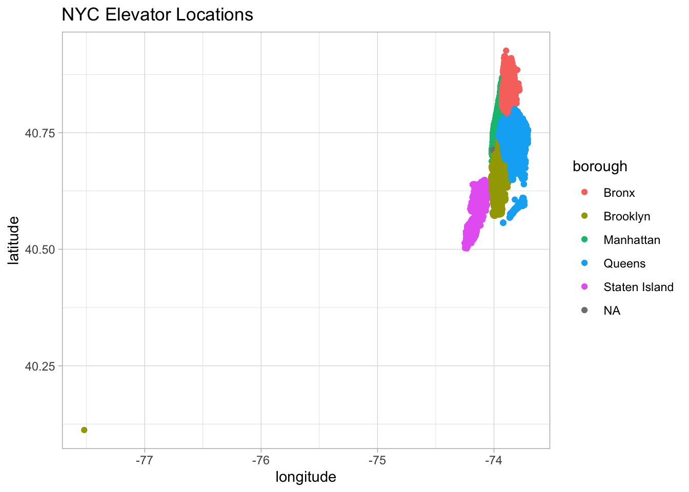

Clean data

I’m gullible, but not that gullible: there shouldn’t be elevators that are 912 stories tall or in the middle of the ocean. Let’s clean this up.

elevators <- tt$elevators %>%
  janitor::clean_names() %>% # Make column names snake_case
  rename_all(str_remove, "^dv_") %>% # Remove the "DV_" that starts many column names
  mutate(
    floor_to_raw = floor_to,
    # Force convert to number, introducing NAs
    floor_to = as.numeric(floor_to_raw), 
    # Remove bad datapoints with absurdly high floors
    floor_to = if_else(floor_to > 90, NA, floor_to), 
    # create explicit missing data for missing zipcodes
    zip_code = na_if(zip_code, 0), 
    # Fix incorrectly formatted zips
    zip_code = str_sub(zip_code, 1, 5)) %>% 
  # Exclude a geographic outlier
  filter(longitude > -76) 

Looking at our cleaned data, how tall are these elevators?

elevators %>%
  filter(!is.na(floor_to)) %>%
  mutate(floor_to = as.numeric(floor_to)) %>%
  ggplot(aes(floor_to)) + 
  geom_histogram() +
  scale_x_log10(labels = scales::comma_format(1))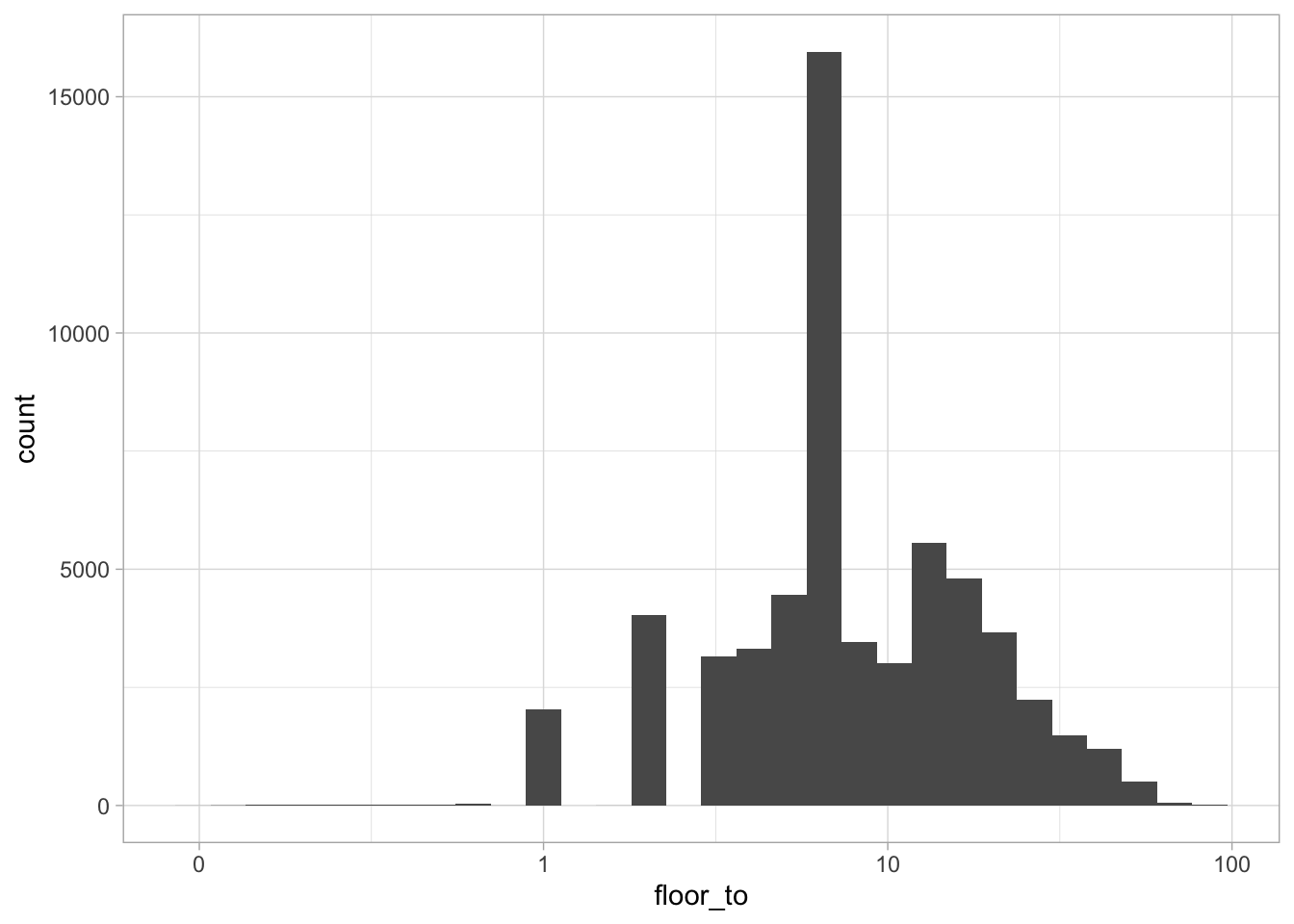

Building heights

Now let’s aggregate by building

by_building <- elevators %>%
  arrange(desc(floor_to)) %>%
  group_by(bin, house_number, street_name, zip_code, borough, longitude, latitude) %>%
  summarize(
    max_floor = na_if(max(floor_to, na.rm = T), -Inf),
    n_elevators = n(),
    latitude = mean(latitude, na.rm = T),
    longitude = mean(longitude, na.rm = T),
    .groups = "drop") %>%
  arrange(desc(max_floor)) 

g <- by_building %>%
  filter(!is.na(max_floor)) %>%
  arrange(max_floor) %>%
  ggplot(aes(longitude, latitude, color = max_floor)) +
  geom_point() +
  scale_color_gradient2(
    trans = "log10",
    low = "blue",
    high = "red",
    midpoint = log10(10)
  ) + 
  ggthemes::theme_map() + 
  theme(
    legend.position = "inside",
    legend.position.inside = c(0.05, 0.75)) +
  labs(
    title = "Height of NYC elevators",
    color = "Max floor")

g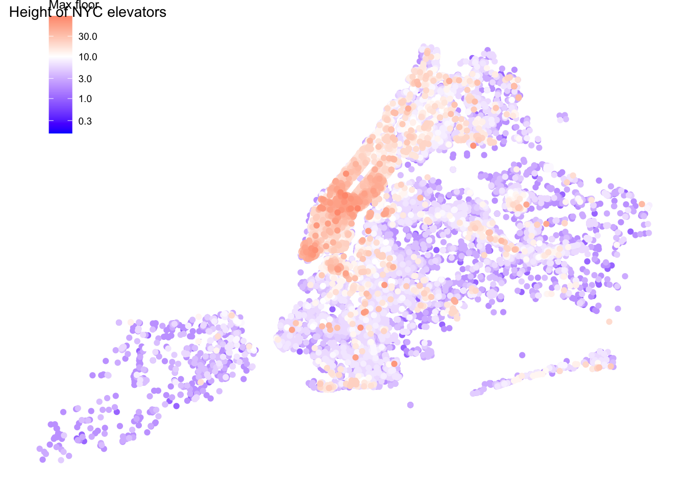

Let’s make this 3D!

library(rayshader)
library(rgl)

plot_gg(
  g, 
  multicore = T, # Use more cores for faster rendering
  # width = 6,     # Increase this (inches) for higher resolution
  # height = 6,    # Increase this (inches) for higher resolution
  scale = 400    # Increase this for more pronounced elevation scaling
)
rglwidget()

Elevator heights by zip code

Join in zip code data to explore elevator heights by zip

library(sf)

zip_codes <- read_sf("data/Modified Zip Code Tabulation Areas (MODZCTA)_20250310")

by_zip_code <- by_building %>%
 filter(!is.na(zip_code)) %>%
 group_by(zip_code, borough) %>%
 summarize(
   n_buildings = n(),
   # geometric mean is a better measure of central tendency 
   #  because the elevator heights are log-normal
   geom_mean_height = exp(mean(log(max_floor), na.rm = T)),
   tallest_building = max(max_floor, na.rm = T),
   .groups = "drop") %>%
 filter(n_buildings >= 20) %>%
 arrange(desc(geom_mean_height))

joined_zip_codes <- zip_codes %>%
 left_join(by_zip_code, by = c("modzcta" = "zip_code"))
 # mutate(
 #   elevator_building_density = n_buildings / pop_est)

joined_zip_codes %>%
 ggplot(aes(fill = geom_mean_height)) +
 geom_sf() +
 scale_fill_gradient2(
   low = "blue",
   high = "red",
   midpoint = log10(6),
   trans = "log10") +
 ggthemes::theme_map() +
 coord_sf(datum = NA) +
  theme(
    legend.position = "inside",
    legend.position.inside = c(0.05, 0.7)) +
 labs(
   title = "Tallest zip codes in NYC",
   fill = "Average (geometric) height of elevators") 

Elevator heights by borough

How do elevator heights vary by borough?

by_building %>%
  filter(!is.na(borough)) %>%
  ggplot(aes(max_floor, borough)) +
  geom_boxplot() + 
  scale_x_log10()

And for folks less familiar with boxplots, here is the same data presented as densities:

by_building %>%
  filter(!is.na(borough)) %>%
  ggplot(aes(max_floor, borough)) +
  geom_violin() + 
  scale_x_log10()

Elevator speed

elevators %>%
  mutate(floor_from = as.numeric(floor_from)) %>%
  ggplot(aes(floor_to - floor_from, parse_number(speed_fpm))) +
  geom_point() +
  scale_x_log10() +
  scale_y_log10() +
  labs(
    title = "Elevator heights vs speed",
    x = "Elevator height (floors)",
    y = "Speed (fpm)")

You can see elevator speeds appear to be correlated with height. In a future analysis, we could find the elevators that are unusual, either unnecessarily fast or too slow given their height.